Midterm 2 - BIOL 480/510/630

0001/01/01

Fall 2020. M Hallett and A Eftyhios

The midterm must be submitted by 2:30pm on Thursday October, 29th, 2020 to \({\tt biol480.concordia@gmail.com}\)

All answers in one email.

Subject header of email is Midterm 2, Lastname, Firstname, student ID.

You can use whichever media you prefer to answer your questions.

This is open book, so you can use whatever resources you would like, but you must cite them. You are not allowed to speak to each other or other experts in this field (eg students who previously took the course). Your sources of information must be cited.

\({\bf 75}\) total marks. (The mditerm is worth \(7.5%\) of your overall grade.)

Question 1 [6 points] In Lecture 07, I introduced the two-dimensional axis for classifying different bioinformatics databases. The “west” extreme represented pure repositories whereas the “east” represented highly curated databases. The “north” represented systems that offered no capacity to run queries on the databases. The “south” represented flexible systems that allow users to design any query they would like.

In the Lecture 07 discussion, we enumerated together reasons why repositories (west) are important.

Why are highly curated databases with the flexible tools to query the contents of these databases important? (“south-east”)

Point form is fine.

Question 2 [4 points] Besides the development and maintenance of databases, what are the primary mandates of bionformatics? (That is, what are the main goals of the field?)

Question 3 [9 points] Approximately one sentence each.

Part A [3 points] What is the difference between a GI and an Accession number at the NCBI?

Part B [3 points] What is the difference between RefSeq and GenBank?

Part C [3 points] What kind of sequence has an accession number that starts with \({\tt NM\_}\) at the NCBI?

Question 4 [10 points] Approximately one sentence each.

Part A [3 points] Give one weakness of metagenomic approaches based on sequencing just the rRNA 16S subunit versus whole genome sequencing “shotgun” approaches discussed in L08.

Part B [3 points] Why did the Tara Oceans project filter large organisms from their samples before whole genome shotgun sequencing?

Part C [2 points] We introduced the use of the Unix \({\tt wget}\) function. Why can \({\tt wget}\) be important to use especially in cloud-based settings like RStudio Cloud?

Part D [2 points] What is Unix?

Question 5 [8 points]

Create a list called \({\tt the\_immortals}\) that produces the following output for the three statements below.

the_immortals$Movie
## [[1]]
## [1] "Iam"
## 
## [[2]]
## [1] "Deadpool"
## 
## [[3]]
## [1] "Deadpool"

the_immortals$TV
## [[1]]
## [1] "Les"
## 
## [[2]]
## [1] "Stroud"
## 
## [[3]]
## [1] "Survivorman"

the_immortals$Reality
## [[1]]
## [1] "Daryl"
## 
## [[2]]
## [1] "Dixon"
## 
## [[3]]
## [1] "Walking Dead"

the_immortals <- list( 
  list(
    "Iam", "Deadpool", "Deadpool"
  ), 
  list(
    "Les", "Stroud", "Survivorman" 
  ),
  list( 
    "Daryl", "Dixon", "Walking Dead"
    )
  )

names(the_immortals) <- c("Movie", "TV", "Reality")  # other ways are possible too.

Question 6 [8 points]

The following questions assume you have a tibble with seven columns as follows:

print(Tara_measure[, c(1:4)])
## # A tibble: 2 x 4
##   pangea_id `latitude:longitude` depth temp_first
##       <dbl> <chr>                <chr>      <dbl>
## 1         1 -13.0:96.0           57.6        20.6
## 2         2 -5.27:-85.2          45.7        19.6
print(Tara_measure[, c(5:7)])
## # A tibble: 2 x 3
##   temp_second salinity_first salinity_second
##         <dbl>          <dbl>           <dbl>
## 1        20.7           35.4            35.3
## 2        19.8           34.7            34.4

You can assume that there are many observations (rows), although only the first two are included here. It is a modified version of the \({\tt Tara}\) tibble we developed in class, but here \({\tt temp\_first}\) and \({\tt temp\_second}\) represent two replicate measurements at the same site. This is also true for the \({\tt salinity}\) variables.

Part A [4 points] Do any of the variables not have the correct class? Provide a sentence justifying your answer. Provide code to modify the class of each variable (or variables) accordingly.

Tara_measure$depth <- as.numeric( Tara_measure$depth)
Tara_measure <- Tara_measure %>% separate( col = 'latitude:longitude', into=c("latitude", "longtitude"), sep = ":")

Part B [4 points] Identify three aspects of \({\tt Tara\_measure}\) that arguably violate the principles of tidy data. Justify your answers with one sentence each. Show code to modify the tibble to make it tidy.

Tara_measure <- Tara_measure %>%
  pivot_longer(c("temp_first", "temp_second"),
                            names_to = "temp_measurement_point",
                            values_to = "temp") %>%
  pivot_longer(c("salinity_first", "salinity_second"),
                            names_to = "salinity_measurement_point",
                            values_to = "salinity")

Question 7 [8 points]

You also have access to this tibble which records the results of the metageomics sequencing that was conducted at each location just once (the sequencing was not replicated). Columns \(2\) and \(3\) correspond to the \({\tt pangea\_id}\) but you can assume there are many additional columns, although they are not shown here.

print(Tara_seq, n=Inf)
## # A tibble: 4 x 3
##   Taxon                   `1`   `2`
##   <chr>                 <dbl> <dbl>
## 1 Alpha_Proteo_Bacteria  1521  2339
## 2 Beta_Proteo_Bacteria    923   458
## 3 Gamma_Proteo_Bacteria  5928  2422
## 4 Cyanobacteria           411   987
tmp <- Tara_seq %>%
  filter(str_detect(Taxon, "Proteo_Bacteria")) %>%
  summarise_at(c('1', '2'), sum) 

tmp <- as.numeric(tmp)
Tara_seq <- add_row( Tara_seq, Taxon = "Proteo_bacteria", '1'= tmp[1], '2' = tmp[2] )

tmp <- Tara_seq %>%
  summarise_at(c('1', '2'), sum) 
tmp <- as.numeric(tmp)

Tara_seq <- add_row( Tara_seq, Taxon = "Bacteria", '1'= tmp[1], '2' = tmp[2] )  # there are lots of other ways to do it.

The first row corresponds to counts for alphaproteobacteria, the second for betaproteobacteria and the third for gammaproteobacteria. These are all proteobacteria.

Show code to add an observation (row) for \({\tt Proteo\_bacteria}\). The counts at sites \(1\) and \(2\) should be the sum over all three sub-categories of proteobacteria.

Similarly, add an observation for \({\tt Bacteria}\) which is the sum of counts over all observed taxa at each site.

Question 8 [10 points]

Show how to join tibbles \({\tt Tara\_measure}\) with \({\tt Tara\_seq}\).

Tara_seq <- Tara_seq %>%
  pivot_longer(cols = !"Taxon", names_to = "pangea_id", values_to = "count") %>%
  pivot_wider(names_from = Taxon, values_from = count)
Tara_measure$pangea_id <- as.character(Tara_measure$pangea_id)  # a small technical thing that I did not remove points for.
Tara_measure_seq <- full_join(Tara_measure, Tara_seq, by = "pangea_id")

Question 9 [12 points]

In Lecture 12, we wrangled the yeast genome (S. cerevisiae) into a tibble and we wrangled the annotations of the genome into a second tibble. We can load these files in project \({\tt L12-Genome~Annotations}\) as follows:

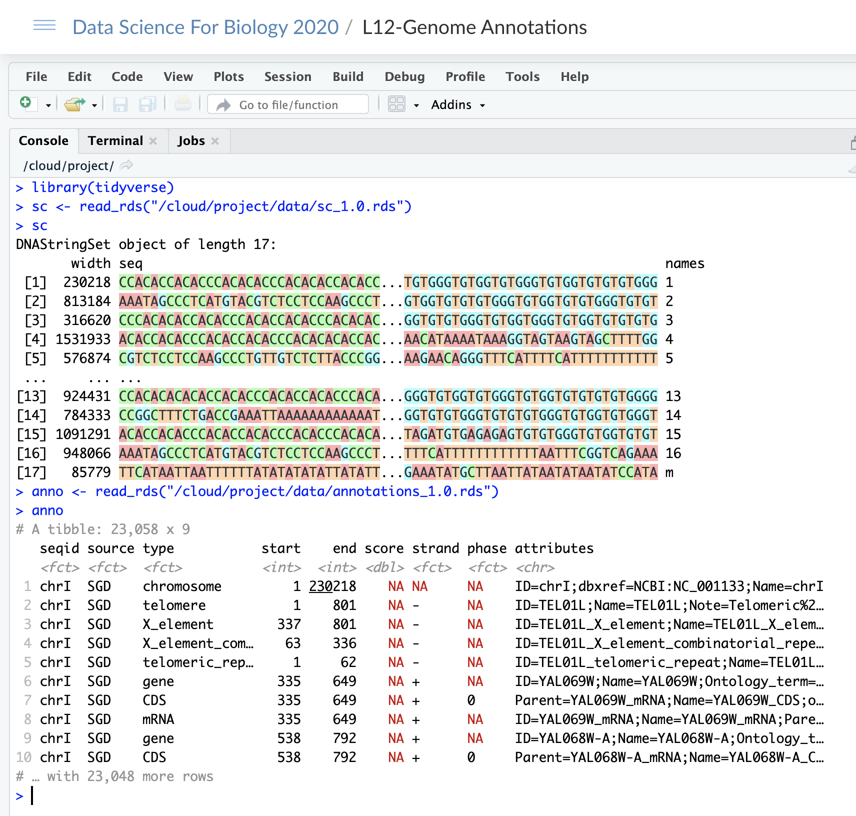
Yeast

Write code that creates a new \({\tt DNAStringSet}\) object called \({\tt coding\_regions}\). Each entry in \({\tt coding\_regions}\) contains the nucleic acid sequence from \({\tt start}\) to \({\tt end}\) for each observation (row) in \({\tt anno}\) that is of type \({\tt gene}\). (Notice that \({\tt type}\) is the name of the third column in \({\tt anno}\).

For example, observation \(6\) of \({\tt anno}\) corresponds to a gene on chromosome \(1\) that starts at position \(335\) and ends at position \(649\). The enty in \({\tt coding\_regions}\) would contain this nucelic acid sequence.

For full marks, create a function which takes two parameters: \({\tt genome}\), which is a \({\tt DNAStringSet}\) object that contains the yeast genome (eg \({\tt sc}\)), and \({\tt annotations}\) which is a tibble that contains all the genome annotations (eg. \({\tt anno}\)). The function returns the \({\tt DNAStringSet}\) object that contains the coding region of each gene.

coding <- function( genome, annotations ) {
  
  levels(annotations$seqid) <- c(1:16, 0)         # I actually forgot that to change this for you; wasn't expecting a  solution for it.
  genes <- annotations %>% filter( type == "gene") 
  
  coding_regions <- DNAStringSet()
  
  for (i in 1:nrow(genes)) {
    chr <- as.numeric(genes[i, "seqid"]); start <- as.numeric(genes[i, "start"]); end <- as.numeric(genes[i, "end"])   # the conversion to numeric was not something i graded. 
    coding_regions[i] <- str_sub( genome[chr], start, end) 
  } # end of for
  
  return(coding_regions)
} # end of coding

Good luck!

© M Hallett, 2020 Concordia University